MeshCNN (ranahanocka.github.io) Siggraph 2019

等变卷积运算、不变的输入特征和学习到的网格池化运算使MeshCNN成为一个特别有趣的模型，它有以下几个主要优点:

• 比旧方法更高效，参数更少；
• 利用网格的拓扑结构(即顶点和面信息)，而不是将其视为点云；
• 网格卷积保留了卷积的便利性质，但允许应用于图形数据。三维网格的5个输入特征类似于输入图像的RGB特征；
• 对旋转、平移和缩放不变性；
• 网格池化(即学习到的边折叠)允许网络通过将5条边折叠成2条边并同时分解两个面来学习特定任务的池化。

Overview

Invariant convolution

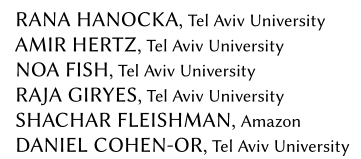
在我们的设置中，假设所有形状都表示为流形网格，可能具有边界边缘。这样的假设保证每条边最多与两个面（三角形）相关，因此与两个或四个其他边相邻。面的顶点按逆时针顺序排序，为每条边的四个邻居定义两种可能的排序。例如，请参见图 4，其中 e 的 1 环邻居可以排序为 (a,b,c,d) 或 (c,d,a,b)，具体取决于哪个面定义第一个邻居。这使得卷积感受野变得模糊，阻碍了不变特征的形成。

我们采取两项措施来解决这个问题，并保证网络内相似变换（旋转、平移和缩放）的不变性。

• 首先，我们仔细设计边缘的输入描述符，使其仅包含对相似变换本质上不变的相对几何特征。
• 其次，我们将四个 1 环边聚合成两对具有模糊性的边（例如，a 和 c，以及 b 和 d），并通过在每对上应用简单的对称函数来生成新特征（例如，sum(a,c)）。

卷积应用于新的对称特征，从而消除任何顺序模糊性。

manifold meshes: 流形网络：

流形学习（Manifold Learning） - 知乎 (zhihu.com)

什么是流形（manifold）、流形学习_Rolandxxx的博客-CSDN博客

对流形（Manifold）的最简单快速的理解_梧桐雪的博客-CSDN博客

2 曲面表示法 - 孙小鸟 - 博客园 (cnblogs.com)

群，李群

Mesh convolution

$$(e^1,e^2,e^3,e^4)=(|a-c|,a+c,|b-d|,b+d)$$

1. 特征提取不用 conv？
2. 如何构建特征？本文为什么这样构建
3. 点边结合（面）

# Simplified from models/layers/mesh_conv.py in ranahanocka/MeshCNN 
 
class MeshCov(nn.Module): 
  def __init__(self, in_c, out_c, k=5, bias=True): 
    super(MeshConv, self).__init__() 
    self.conv = nn.Conv2d(in_channels=in_c, out_channels=out_c, kernel_size=(1, k), bias=bias)
########    self.transformer = nn.transformer( )??????????
    
 
  def forward(self, x) 
    """ 
      Forward pass given a feature tensor x with shape (N, C, E, 5): 
        N - batch 
        C - # features 
        E - # edges in mesh 
        5 - edges in neighborhood (0 is central edge) 
    """ 
    x_1 = x[:, :, :, 1] + x[:, :, :, 3] 
    x_2 = x[:, :, :, 2] + x[:, :, :, 4] 
    x_3 = torch.abs(x[:, :, :, 1] - x[:, :, :, 3]) 
    x_4 = torch.abs(x[:, :, :, 2] - x[:, :, :, 4]) 
    x = torch.stack([x[:, :, :, 0], x_1, x_2, x_3, x_4], dim=3) 
    x = self.conv(x) 
    return x

torch.cat()

函数目的： 在给定维度上对输入的张量序列seq 进行连接操作。

---

torch.stack() 官方解释：沿着一个新维度对输入张量序列进行连接。 序列中所有的张量都应该为相同形状。

浅显说法：把多个2维的张量凑成一个3维的张量；多个3维的凑成一个4维的张量…以此类推，也就是在增加新的维度进行堆叠。

outputs = torch.stack(inputs, dim=?) → Tensor 参数

inputs : 待连接的张量序列。 注：python的序列数据只有list和tuple。

dim : 新的维度， 必须在0到len(outputs)之间。 注：len(outputs) 是生成数据的维度大小，也就是outputs的维度值。

2. 重点 函数中的输入inputs只允许是序列；且序列内部的张量元素，必须shape相等 ----举例：[tensor_1, tensor_2,..] 或者 (tensor_1, tensor_2,..)，且必须tensor_1.shape == tensor_2.shape

dim 是选择生成的维度，必须满足0<=dim<len(outputs)；len(outputs)是输出后的 tensor 的维度大小 ———————————————— 版权声明：本文为CSDN博主「模糊包」的原创文章，遵循CC 4.0 BY-SA版权协议，转载请附上原文出处链接及本声明。 原文链接：https://blog.csdn.net/xinjieyuan/article/details/105205326

输入特征

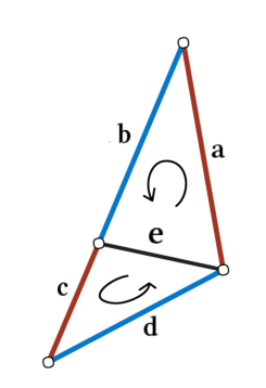
在应用第一次卷积之前，我们必须创建一个类似于二维图像中的RGB通道的输入特征表示。为此，作者简单地为每个面定义了二面角(两个相邻面之间的角)、对称对顶角(相对角的角，排序以保持顺序不变性)和两个边长比(每个三角形的高/基比，也排序)，总共为5个输入特征。

We sort each of the two face-based features (inner angles and edge-length ratios), thereby resolving the ordering ambiguity and guaranteeing invariance. Observe that these features are all relative, making them invariant to translation, rotation and uniform scale.

# From models/layers/mesh_conv.py in ranahanocka/MeshCNN 
 
def dihedral_angle(mesh, edge_points): 
  """ 
  Angle between two faces connected to edge. 
  """ 
  normals_a = get_normals(mesh, edge_points, 0) 
  normals_b = get_normals(mesh, edge_points, 3) 
  dot = np.sum(normals_a * normals_b, axis=1).clip(-1, 1) 
  angles = np.expand_dims(np.pi - np.arccos(dot), axis=0) 
  return angles 
 
def symmetric_opposite_angles(mesh, edge_points): 
  """ 
  Angles of opposite corners across edge. 
  """ 
  angles_a = get_opposite_angles(mesh, edge_points, 0) 
  angles_b = get_opposite_angles(mesh, edge_points, 3) 
  angles = np.concatenate((np.expand_dims(angles_a, 0), np.expand_dims(angles_b, 0)), axis=0) 
  angles = np.sort(angles, axis=0) 
  return angles 
 
def symmetric_ratios(mesh, edge_points): 
  """ 
  Height/base ratios of the triangles adjacent to edge. 
  """ 
  ratios_a = get_ratios(mesh, edge_points, 0) 
  ratios_b = get_ratios(mesh, edge_points, 3) 
  ratios = np.concatenate((np.expand_dims(ratios_a, 0), np.expand_dims(ratios_b, 0)), axis=0) 
  return np.sort(ratios, axis=0)

Global ordering

数据是按一个特定顺序输入网络的，但因为卷积作用于邻域输入顺序在卷积阶段不产生影响。进一步说，分割任务也不受它的影响。对于需要全局特征聚合的任务，例如分类，作者遵循Qi 等人在PointNet中提出的常用做法，并在卷积部分和网络的全连接部分之间放置一个全局平均池化层。这样做保证了结果与输入顺序无关，也保证了转换不变性。

Pooling

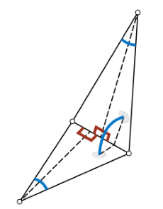
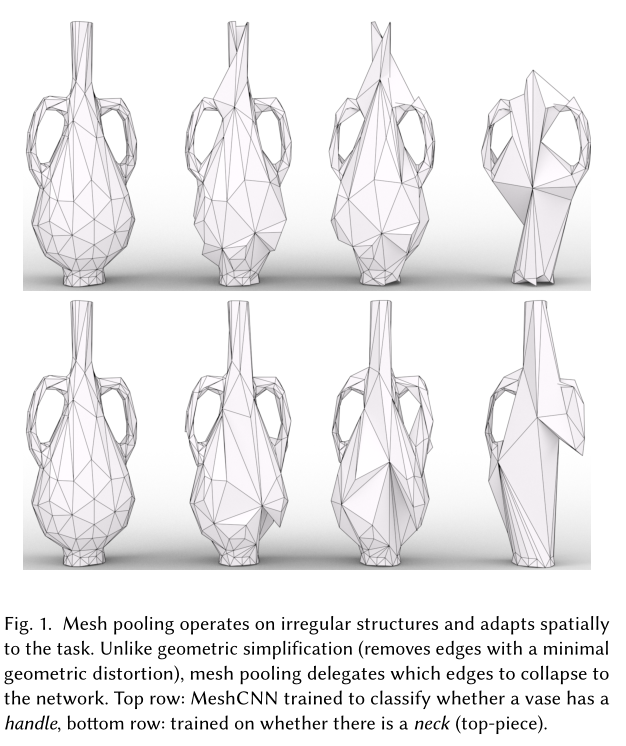
网格池是通过边缘折叠过程完成的，如图 2 (b) 和 (c) 所示。在 (b) 中，虚线边缘折叠成一个点，随后，四个入射边缘（蓝色）合并为 (c) 中的两个（蓝色）边缘。

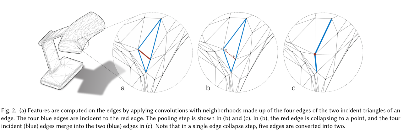
请注意，在此边缘折叠操作中，五个边缘转换为两个。算子按（最小范数）边缘特征确定优先级，从而允许网络选择网格的哪些部分要简化，哪些部分保持不变。这创建了一个任务感知过程，其中网络学习确定对象部分相对于其任务的重要性（见图 1）。

Mesh Pooling

1)定义给定邻接的池化区域 2)合并每个池化区域中的特征 3)重新定义合并特征的邻接关系

网格池化是广义池化的另一种特殊情况，其中邻接关系由拓扑结构决定。作者将网格池化定义为一系列的边折叠操作，其中每个边折叠将5条边转换为2条边。因此，可以通过添加一个超参数来定义池化网格中目标边缘的数量，从而在每个池化操作之后控制网格的期望分辨率。 根据边缘特征的大小对边折叠顺序(使用优先队列)进行优先级排序，允许网络选择网格的哪些部分与解决任务相关。这使得网络能够非均匀地折叠某些对损失影响最小的区域。通过对每个特征通道取平均值，每个面三个边缘的每个特征被合并为一个新的边缘特征。 根据边的特征强度对边折叠进行优先级排序，该特征强度作为边折叠的L2范数。如图5所示，特征被聚合，其中有两个合并操作，一个针对最小边特征e的每个关联三角形，产生两个新的特征向量(表示为p和q)。边在每个i通道中的特征p由以下公式给出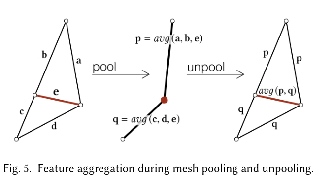

并不是所有的边都可以折叠。在作者的设置中，不允许产生非流形面的边缘折叠，因为它违反了四个卷积邻居的假设。

Mesh UnPooling

Unpooling is the (partial) inverse of the pooling operation. While pooling layers reduce the resolution of the feature activations (encoding or compressing information), unpooling layers increase the resolution of the feature activations (decoding or uncompressing information). The pooling operation records the history from the merge operations (e.g., max locations), and uses them to expand the feature activation. Thus, unpooling does not have learnable parameters, and it is typically combined with convolutions to recover the original resolution lost in the pooling operation. The combination with the convolution effectively makes the unpooling a learnable operation.

Each mesh unpooling layer is paired with a mesh pooling layer, to upsample the mesh topology and the edge features. The unpooling layer reinstates the upsampled topology (prior to mesh pooling), by storing the connectivity prior to pooling. Note that upsampling the connectivity is a reversible operation (just as in images). For unpooled edge feature computation, we retain a graph which stores the adjacencies from the original edges (prior to pooling) to the new edges (after pooling). Each unpooled edge feature is then a weighted combination of the pooled edge features. The case of average unpooling is demonstrated in Figure 5.

反池化（反卷积）是一个可学习的过程吗？

反卷积详解_bestrivern的博客-CSDN博客

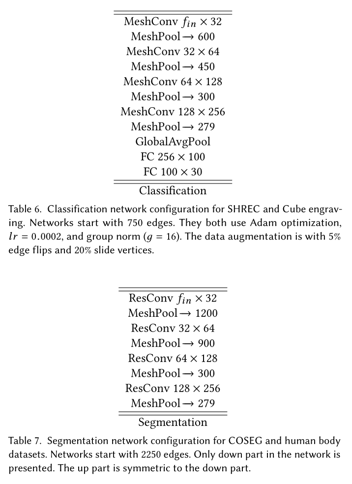
网络设置

网络结构由MResConv层组成，每个层由一个初始网格卷积(MeshConv)、几个连续的ReLU+BatchNorm+MeshConv层和一个残差连接和另一个ReLU组成。在任务层结束之前，网络遵循多次MResConv+Norm+MeshPool的模式。对于分类，任务层是简单的全局平均池化，然后是两个完全连接的层。分割网络是一个U-Net风格的编码器-解码器。

Result

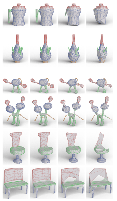
（保留的）测试形状的语义分割结果。每个边缘的分割预测显示在左侧，后面是每个池化层之后的中间简化网格。出于可视化目的，中间网格中的边缘使用最终分割预测进行着色。 MeshCNN 使用网格池来学习折叠来自相同片段的边缘，这些边缘通过网格反池化层展开回原始输入网格分辨率（例如，请参见顶行，其中整个花瓶手柄已折叠为单个边缘）。

总结

本文提出了一种直接在不规则三角网格上使用神经网络的通用方法MeshCNN。本文工作的关键贡献是针对不规则和非均匀结构定制的卷积和池化操作的定义和应用。作者通过利用三角网格特有的对称性，消除邻居排序对偶的歧义，以实现变换的不变性的构思很巧妙。作者通过边折叠的方式来进行池化，通过池化聚合了局部特征信息，也通过边折叠的方式在最小化损失信息的基础上，将卷积的邻域扩大了，在更大的尺度上聚合特征信息。

MeshCNN与PointNet++的一些差别：

• MeshCNN的下采样与task的相关性更高：PointNet++在下卷积时通过FPS（farthest point sampling）的方式选择下一层的中心点，因此点的选择基本只依赖于mesh本身的结构，与task的关系不大，也就是说无论mesh被用于什么task，下卷积的采样中心是基本一致的。但MeshCNN的下采样是与具体task密切相关的，它能够在下采样的时候，更多地保留与task密切相关的边，这一点与图像中的max pooling具有更相似的内在含义。
• MeshCNN的上采样与下采样的结构一致性更强：MeshCNN和PointNet都采用了类似UNet的结构。但相比MeshCNN直接用下采样的mesh结构来进行上采样，PointNet++中的上采样和下采样的感知域是不一样的，以scannet数据集为例，下采样是邻域32个点，上采样是邻域3个点。
• MeshCNN的感知域在模型表面空间：PointNet++使用knn挑选空间距离上的领域点，这种方式有可能采样到测地距离远但空间距离近的点。而MeshCNN根据边进行上下采样，更接近于挑选测地距离上的领域，感知域在模型表面空间。

稀疏卷积：稀疏卷积 Sparse Convolution Net - 知乎 (zhihu.com)

Minkowski Convolutional Neural Networks：NVIDIA/MinkowskiEngine: Minkowski Engine is an auto-diff neural network library for high-dimensional sparse tensors (github.com)